Configuring and Installing TensorFlow for Non-Titan GPUs

TensorFlow officially supports GPUs with versions greater than the GeForce GTX TITAN. However, it is possible to configure and install TensorFlow for GPUs before Titan, such as the GeForce GTX 960 (which I have used for verification) by using "unofficial settings" that are not tested and supported (but is mentioned on the official installation instructions).

TensorFlow's official GPU compatibility is mentioned in the "Optional: Install CUDA (GPUs on Linux)" section in the TensorFlow installation instructions
https://www.tensorflow.org/get_started/os_setup.html#installation-for-linux:

TensorFlow GPU support requires having a GPU card with NVidia Compute Capability >= 3.5. Supported cards include but are not limited to:

However, as mentioned in the "Enabling Cuda 3.0" section, we can configure and install TensorFlow for non-Titan GPUs by using "unofficial settings" during the configuration.

Caution: as it is called as "unofficial," this method is "largely untested and unsupported," meaning that the installation may be glitchy. This is mentioned in the following message that appears during the `./configure` part in the installation:

WARNING: You are configuring unofficial settings in TensorFlow. Because some
external libraries are not backward compatible, these settings are largely
untested and unsupported.

A Japanese version of this entry can be found here: http://qiita.com/woodrush/items/67703153541ce869e3dc

Installation

Build from source, according to the official installation guide
https://www.tensorflow.org/versions/master/get_started/os_setup.html:

  1. Follow each step in the "Installing from sources" section before the "Configure the installation" step
  2. Follow the "Enabling Cuda 3.0" section and ./configure the "unofficial settings"
  3. Follow the "Create the pip package and install" to create a pip wheel and install TensorFlow from the wheel
    • (This step is required only when installing in virtual python environments such as pyenv, virtualenv, etc. When installing TensorFlow for the system's Python environment, follow the instructions in "Build your target with GPU support" section instead.)

I used a Geforce GTX 960, Ubuntu 15.04 PC setup for verifying these steps. I tested the "Neural Art in TensorFlow" repo for testing functionality: woodrush/neural-art-tf · GitHub.
tmuxの使い方:一晩サーバーに仕事を投げて、翌日結果を見たい!

「一晩サーバーに仕事を投げて、翌日結果を見たい!」
「学校でサーバーにタスクを投げて、後で家で確認したい!」
Windows Updateが始まってssh接続が切れてしまった…つらい…」

こんな場面はしばしばあります。普通にssh接続をしている場合、接続を切るとタスクが止まってしまいます。すると上記のような場合、sshで接続している自機を一晩中つけておいたり、学校から家までsshの接続をずっと保っておくわけには行きません。Windows Updateなどで強制的にsshが切られたらもっと嫌です。

そんな時にはtmuxを使います。tmuxはかなり多くの機能があるのですが、上記の用途だけなら2, 3個コマンドを覚えるだけで十分です。

tmuxの詳しい動作原理はtmuxを使い始めたので基本的な機能の使い方とかを整理してみた - 完熟トマトの「tmux利用のイメージ図」がわかりやすいです。ごく簡単に言うと、tmuxはサーバー側に仮想端末を包み込んだ(アタッチした)プロセスを走らせておきます。この仮想端末はsshを切っても裏で動き続けてくれるので、一晩寝ていても裏でタスクを走らせ続けることができるのです。

tmuxの使い方については主に下記のサイトを参考にしました。
tmuxを使い始めたので基本的な機能の使い方とかを整理してみた - 完熟トマト
www.task-notes.com

1. サーバー側でtmuxをインストール

まずはターミナルからtmuxをインストールします。

Ubuntuの場合、下記でインストールします:

sudo apt-get install tmux

これでインストール出来ない場合はtmux installation steps for Ubuntu · GitHubが参考になるかもしれません。

Mac OS Xの場合、Homebrewをインストールした状態で下記でインストールします:

brew install tmux

また、tmuxを使い始めたので基本的な機能の使い方とかを整理してみた - 完熟トマトによると、RHELLinuxでは「EPELリポジトリにパッケージが存在しますのでyumでパッケージをインストールできます」:

yum install http://dl.fedoraproject.org/pub/epel/6/x86_64/tmux-1.6-3.el6.x86_64.rpm

また、tmuxの基本的な使い方とコマンドのまとめ - TASK NOTESによると、CentOSの場合は「EPELリポジトリを追加してインストールします」:

rpm -i http://ftp.riken.jp/Linux/fedora/epel/6/x86_64/epel-release-6-8.noarch.rpm
yum -y install tmux

2. 作業開始:tmuxを起動

いよいよtmuxを使います。まず、sshで処理を行いたいサーバーへ接続します。そして、

tmux

を実行します。すると、仮想端末(セッション)が開始します。

仮想端末は閉じたり開いたりするので、名前をつけておきます。そのためには「Control - b」「$」と続けて押します。(Controlで操作するのはemacsに似ていますね。)その後、セッション名を入力してEnterで名前がつきます。

tmux起動と同時にセッションに名前を付けるには

tmux new-session -s <session-name>

とします。

さて、名前のついたセッションを起動しました。セッションは普通の端末と同じように使えるので、一晩投げたいタスクをここで実行します。

3. 作業中断:セッションのデタッチ

タスクも実行開始した所で、いよいよ一晩寝る時がやってきました。セッションをデタッチするには、「Control - b」「d」と続けて押します。すると、仮想端末から抜けて普通の端末に戻ります。
しかし、裏ではtmuxの仮想端末がちゃんと動いています。この普通の端末で

tmux ls

を実行してみましょう。すると、先ほど名前をつけた端末が裏で走っています。

デタッチしたセッションを再びアタッチするには、

tmux a -t <session-name>

とします。これで、先ほどの処理の実行途中でも、その端末の様子を見ることが出来ます。

ここでサーバーとのssh接続を切って、再び接続し、同じくtmux lsを実行しても、やはり裏で仮想端末が走り続けてくれています。
これで、安心して一晩寝ることが出来ます。

4. 作業復帰:セッションのアタッチ

新しい朝がやって来ました。進捗確認のため、サーバーにsshで接続し、先ほどのように

tmux a -t <session-name>

を実行します。セッション名を忘れたらtmux lsで確認すれば大丈夫です。

これで一晩寝られる!

これで、あなたもサーバーにタスクを投げて一晩寝られるようになりました。

tmuxにはここで紹介した他にも色々な便利な機能があります。詳しくは、
tmuxを使い始めたので基本的な機能の使い方とかを整理してみた - 完熟トマト
tmuxの基本的な使い方とコマンドのまとめ - TASK NOTES
が大変参考になります。

Installing Torch (OpenBLAS) on Ubuntu 15.04 with Skylake CPUs

As I encountered a problem installing Torch in Ubuntu 15.04 probably because of using Skylake CPUs (Intel Core i7 6600), I would like to share how I have managed installing it on my system. The main reasons were installation errors of OpenBLAS and luacrypto.

My system setup is as follows:
MB: z170 Extreme 6 (with z170 chipset)
CPU: Intel Core i7 6600
OS: Ubuntu 15.04 Japanese Remix

I was installing Torch as said on its official website:
Torch | Getting started with Torch
Installation failed on the following command:

curl -s https://raw.githubusercontent.com/torch/ezinstall/master/install-deps | bash

With the following error indicating OpenBLAS was not compiled:

Cloning into 'OpenBLAS'...
remote: Counting objects: 17300, done.
remote: Compressing objects: 100% (8/8), done.
remote: Total 17300 (delta 2), reused 0 (delta 0), pack-reused 17292
Receiving objects: 100% (17300/17300), 14.80 MiB | 3.03 MiB/s, done.
Resolving deltas: 100% (11998/11998), done.
Checking connectivity... done.
getarch_2nd.c: In function ‘main’:
getarch_2nd.c:12:35: error: ‘SGEMM_DEFAULT_UNROLL_M’ undeclared (first use in this function)
printf("SGEMM_UNROLL_M=%d\n", SGEMM_DEFAULT_UNROLL_M);
^
getarch_2nd.c:12:35: note: each undeclared identifier is reported only once for each function it appears in
getarch_2nd.c:13:35: error: ‘SGEMM_DEFAULT_UNROLL_N’ undeclared (first use in this function)
printf("SGEMM_UNROLL_N=%d\n", SGEMM_DEFAULT_UNROLL_N);
^
getarch_2nd.c:14:35: error: ‘DGEMM_DEFAULT_UNROLL_M’ undeclared (first use in this function)
printf("DGEMM_UNROLL_M=%d\n", DGEMM_DEFAULT_UNROLL_M);
^
getarch_2nd.c:15:35: error: ‘DGEMM_DEFAULT_UNROLL_N’ undeclared (first use in this function)
printf("DGEMM_UNROLL_N=%d\n", DGEMM_DEFAULT_UNROLL_N);
^
getarch_2nd.c:19:35: error: ‘CGEMM_DEFAULT_UNROLL_M’ undeclared (first use in this function)
printf("CGEMM_UNROLL_M=%d\n", CGEMM_DEFAULT_UNROLL_M);
^
getarch_2nd.c:20:35: error: ‘CGEMM_DEFAULT_UNROLL_N’ undeclared (first use in this function)
printf("CGEMM_UNROLL_N=%d\n", CGEMM_DEFAULT_UNROLL_N);
^
getarch_2nd.c:21:35: error: ‘ZGEMM_DEFAULT_UNROLL_M’ undeclared (first use in this function)
printf("ZGEMM_UNROLL_M=%d\n", ZGEMM_DEFAULT_UNROLL_M);
^
getarch_2nd.c:22:35: error: ‘ZGEMM_DEFAULT_UNROLL_N’ undeclared (first use in this function)
printf("ZGEMM_UNROLL_N=%d\n", ZGEMM_DEFAULT_UNROLL_N);
^
getarch_2nd.c:67:50: error: ‘SGEMM_DEFAULT_Q’ undeclared (first use in this function)
printf("#define SLOCAL_BUFFER_SIZE\t%ld\n", (SGEMM_DEFAULT_Q * SGEMM_DEFAULT_UNROLL_N * 4 * 1 * sizeof(float)));
^
getarch_2nd.c:68:50: error: ‘DGEMM_DEFAULT_Q’ undeclared (first use in this function)
printf("#define DLOCAL_BUFFER_SIZE\t%ld\n", (DGEMM_DEFAULT_Q * DGEMM_DEFAULT_UNROLL_N * 2 * 1 * sizeof(double)));
^
getarch_2nd.c:69:50: error: ‘CGEMM_DEFAULT_Q’ undeclared (first use in this function)
printf("#define CLOCAL_BUFFER_SIZE\t%ld\n", (CGEMM_DEFAULT_Q * CGEMM_DEFAULT_UNROLL_N * 4 * 2 * sizeof(float)));
^
getarch_2nd.c:70:50: error: ‘ZGEMM_DEFAULT_Q’ undeclared (first use in this function)
printf("#define ZLOCAL_BUFFER_SIZE\t%ld\n", (ZGEMM_DEFAULT_Q * ZGEMM_DEFAULT_UNROLL_N * 2 * 2 * sizeof(double)));
^
make: *** [getarch_2nd] Error 1
Makefile:131: *** OpenBLAS: Detecting CPU failed. Please set TARGET explicitly, e.g. make TARGET=your_cpu_target. Please read README for the detail.. 中止.
Error. OpenBLAS could not be compiled

I found the following issue at the OpenBLAS repo:
The build system doesn't know about SkyLake · Issue #632 · xianyi/OpenBLAS · GitHub

martin-frbg commented 25 days ago

"TARGET=BROADWELL" should work on the "develop" branch (which you will probably want to try rather than the already somewhat dated 0.2.14 release)
(Edited to add: judging from cpuid_x86.c, Broadwell cpu is simply mapped to Haswell even in the develop branch, but you will probably still want all the fixes that went in since the 0.2.14 release)

xianyi commented 23 days ago

@yuyichao , I didn't optimize skylake yet. Therefore, please use haswell kernels. make TARGET=HASWELL

So I did

curl -s https://raw.githubusercontent.com/torch/ezinstall/master/install-deps > installtorch.sh

and edited it to create a custom installation shellscript: (edit: deleted lines that specified to use the `develop` branch)

diff installtorch.sh installtorch-new.sh 
14,16c14,16
<         make NO_AFFINITY=1 USE_OPENMP=0 USE_THREAD=0
<     else
<         make NO_AFFINITY=1 USE_OPENMP=1
---
>         make NO_AFFINITY=1 USE_OPENMP=0 USE_THREAD=0 TARGET=HASWELL
>     else 
>         make NO_AFFINITY=1 USE_OPENMP=1 TARGET=HASWELL

This shellscript let OpenBLAS compile correctly, letting the command that failed to pass.

Installing luacrypto

I encountered another failure on the third command,

cd ~/torch; ./install.sh

and got the following error:

Missing dependencies for itorch:
lbase64
luacrypto
uuid
lzmq >= 0.4.2

Using https://raw.githubusercontent.com/rocks-moonscript-org/moonrocks-mirror/master/lbase64-20120820-1.src.rock... switching to 'build' mode
Do not use 'module' as a build type. Use 'builtin' instead.
gcc -O2 -fPIC -I/home/woodrush/torch/install/include -c lbase64.c -o lbase64.o
gcc -shared -o base64.so -L/home/woodrush/torch/install/lib lbase64.o
Updating manifest for /home/woodrush/torch/install/lib/luarocks/rocks
lbase64 20120820-1 is now built and installed in /home/woodrush/torch/install/ (license: Public domain)

Using https://raw.githubusercontent.com/rocks-moonscript-org/moonrocks-mirror/master/luacrypto-0.3.2-1.src.rock... switching to 'build' mode

Error: Failed installing dependency: https://raw.githubusercontent.com/rocks-moonscript-org/moonrocks-mirror/master/luacrypto-0.3.2-1.src.rock - Could not find expected file openssl/evp.h, or openssl/evp.h for OPENSSL -- you may have to install OPENSSL in your system and/or pass OPENSSL_DIR or OPENSSL_INCDIR to the luarocks command. Example: luarocks install luacrypto OPENSSL_DIR=/usr/local

I found the following issue on a different OpenSSL problem:
cmake not able to find openssl - Stack Overflow

so I did

    sudo apt-get install libssl-dev

to make sure I installed luacrypto I also did (may not be necessary)

    sudo apt-get install libssl-dev
    sudo apt-get install luarocks
    source .bashrc       # This was after I failed installing torch with the third command: this seems to have the effect of enabling luarocks
    luarocks install luacrypto

and the rest of the Torch installation finished successfully.

Survey: Marschner, et al. (2003), Light scattering from human hair fibers (The Marschner Model)

As I had an opportunity to read and implement Marschner's paper [1] on the Marschner Model, I would like to share the details and points I have stumbled upon on reading the paper. The Marschner Model is a model proposed in 2003, that describes how light is scattered (reflected and transmitted) in human hair. It is used to implement shaders for human hair models, and rendering realistic hair.
[1] MARSCHNER, S. R., et al., 2003. Light scattering from human hair fibers. ACM Trans. Graph. 22, 3, 780–791. http://www.graphics.stanford.edu/papers/hair/

For conducting this survey, I've also referenced the following blog post:
Marschner Shader Part II | Real-Time Hair Simulation and Rendering


Overview

The Marschner Model is essentially a scattering function {S(\omega_i,\omega_r)}, which lets you find how much light is redirected from one direction to another. Simply put, it is the ratio of incoming light intensity from direction {\omega_i} against the outcoming light intensity from direction {\omega_r}. Given an outcoming direction {\omega_r}, it can be used as

{
\bar L_r(\omega_r) = D \int
S(\omega_i, \omega_r)
L_i(\omega_i)
\cos \theta_i\,
d \omega_i,
}

to determine the amount of light emitted in that direction.

  • Here, {\bar L} is the intensity per *length* (which is different from ordinary *radiance*, which is intensity per *area*), which they call as *curve intensity*.
  • {D} is the diameter of the hair - which implies that outcoming light increases for thicker hair, i.e. thicker hairs are more shiny.
  • One novel point of the Marschner Model is that {S} is a function of only the *direction* of incidence, and not the *position* of incidence, meaning that the hair's thickness is *taken out of thought*. In the derivation, the hair's thickness (the position of ray-hair intersection) is explicitly considered, but is effectively ignored in its final form.


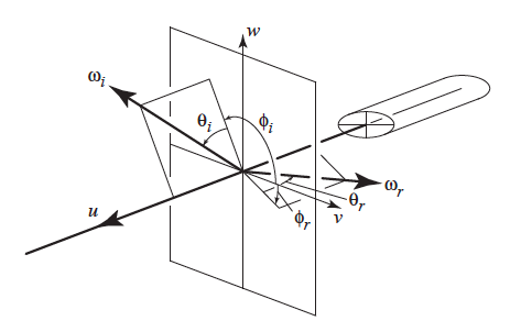
f:id:woodrush:20150923200321p:plain

Figure 1. The coordinate system. Image cited from Marschner, et al. (2003) [1]

One important point that I've stumbled upon is the coordinate system. Although at first sight it seems like an ordinary spherical system with {w} as the {z} direction, that is actually not the case. Here, {\theta_i} and {\theta_r} are measured as the inclination to the {w}-{v} plane. Therefore,

{
\begin{align}
\theta_i &:= \frac \pi 2 - \cos^{-1} (\omega_i \cdot u), \\
\phi_i &:= \tan^{-1} \left(\frac{\omega_i \cdot w}{\omega_i \cdot v}\right). \\
\end{align}
}

The same holds for {\omega_r}.


In the paper, the hair is modeled as an elliptic cylinder with a bumpy surface (which models cuticles). They first start with an ideal, smooth cylinder case, where {S} is given as

{
S(\phi_i, \theta_i ; \phi_r, \theta_r) = \delta(\theta_r + \theta_i) N(\eta'(\theta); \phi_i, \phi_r) / \cos^2 \theta.
}

Where {\delta} is the delta function.
The term {\delta(\theta_r + \theta_i)} implies that scattering only occurs when {\theta_r = \theta_i}, which ultimately implies that an incoming straight ray is emitted in the shape of a cone.

We can see that {S} is decomposed into {\theta}-dependent parts and {\phi}-dependent parts. This is one of the important features of this model, derived from the symmetry of the cylindric geometry of the hair.

The actual Marschner Model is an extention of this equation,

{ 
\begin{align}
S(\phi_i, \theta_i ; \phi_r, \theta_r)
&=M_{R}  (\theta_h) N_{R}  (\eta'(\eta,\theta_d); \phi) / \cos^2 \theta_d \\
&+M_{TT} (\theta_h) N_{TT} (\eta'(\eta,\theta_d); \phi) / \cos^2 \theta_d \\
&+M_{TRT}(\theta_h) N_{TRT}(\eta'(\eta^*(\phi_h),\theta_d); \phi) / \cos^2 \theta_d.
\end{align}
}

Although there are more terms, all emitted light is still contained in a single cone. The 3 terms represent the 3 modes of scattering that are considered (all modes are in the same cone). We can recognize that one major extension is the replacement of {\delta(\theta_r + \theta_i)} with {M(\theta_h)}.

  • {\eta '} is one of the difficult parts of this paper. In this paper, simply put, *3D Fresnel effects are evaluated as 2D Fresnel effects with an augmented index of refraction,* thanks to the symmetry of hair (c.f. p. 6). We know that in Fresnel reflections/refractions, all light paths are contained in one plane. Obviously, this plane does not necessarily run parallel to the surface normal of the hair, and can be tilted (i.e., the plane may not cross the hair orthogonally). In this paper, the "3D" light path (on the tilted plane) is projected on to the plane perpendicular to the hair surface. Then, the Fresnel equations are evaluated *on the projected plane*, and then *projected back to the original tilted plane*. The augmented index of refraction, used on the projected plane, is {\eta '} - which only depends on {\theta} due to the projection.

The Model

{M} is a "unit-integral, zero-mean lobe function with width {\beta}" (c.f. p.8), i.e. simply a probability distribution {g}:

{ 
\begin{align}
M_{R}  (\theta_h) &= g(\alpha_{R}  , \beta_{R}  ;\theta_h) \\
M_{TT} (\theta_h) &= g(\alpha_{TT} , \beta_{TT} ;\theta_h) \\
M_{TRT}(\theta_h) &= g(\alpha_{TRT}, \beta_{TRT};\theta_h) 
\end{align}
}

In the paper, {g(\alpha, \beta, x)} is given as a normalized Gaussian function with mean {\alpha} and standard deviation {\beta}:
{ 
g(\alpha, \beta, x) = \frac 1 {\sqrt{2 \pi \beta^{2}}}
\exp \left(-\frac{(x - \alpha)^2}{2\beta^{2}}
\right).
}

  • The notation for the dependency of {\alpha} on {g} is changed for clarity.

{N} is complicated to find. First, as a notation, the paths {R, TT, TRT} are given an index {p=0,1,2}, respectively. Then:

{ 
\begin{align}
N_p(\eta'(\eta,\theta_d),p,\phi) &:= \sum_{\gamma_i \in \Gamma} A(p,h(p,\gamma_i,\phi))
\left|
	2 \frac {d\hat\phi} {dh}(p, h(p,\gamma_i,\phi))
\right|^{-1}.
\end{align}
}

Here, {\phi := \phi_i - \phi_t}. This means that {N_p} depends on the azimuths through only their *difference*.

  • We have additionally written the {\eta'(\eta,\theta_d)}-dependency of {N_p} and {h}.
  • The notation of the sum and the arguments of {h} were changed for clarity.
  • Confusingly, in the original paper there is a *variable* {\phi := \phi_i - \phi_t/2} and a *function* {\phi(p,\gamma_i)} which are different quantities. {\phi(p,\gamma_i)} is a trigonometric function (c.f. p.6) and is later approximated as {\hat \phi(p,\gamma_i)} (c.f. p.8). For brevity, we will write {\hat \phi} in place of the original function {\phi(p,\gamma_i)}.

Below, we will study the actual forms of each term.


Definition of {\eta'}, {\eta''}:

{\eta'}, {\eta''} are the corrected values of {\eta}:

{ 
\begin{align}
	\eta'(\eta, \varphi)  &:= \sqrt{\eta^2 - \sin^2 \varphi} \Big/ \cos \varphi\\
	\eta''(\eta, \varphi) &:= \eta^2 \cos \varphi \Big/ \sqrt{\eta^2 - \sin ^2 \varphi}
\end{align}
}

Here, {\eta} is a constant (c.f. p.8).

Definition of {F}:

{F} is the corrected Fresnel reflectance function, computed with the corrected refraction indices {\eta', \eta''}.

We know the ordinary Fresnel reflectance functions are given as:

{ 
\begin{align}
	F_s(\eta_1, \eta_2, \varphi)
	&:=
	\frac
	{\eta_1 \cos \varphi - \eta_2 \cos \varphi'}
	{\eta_1 \cos \varphi + \eta_2 \cos \varphi'} \\
	F_t(\eta_1, \eta_2, \varphi)
	&:=
	\frac
	{\eta_1 \cos \varphi' - \eta_2 \cos \varphi}
	{\eta_1 \cos \varphi' + \eta_2 \cos \varphi} \\
	\varphi' &:= \sin^{-1}\left(\frac{\eta_1}{\eta_2}\sin \varphi \right)
\end{align}
}

The corrected Fresnel function {F} is then defined as
{ 
\begin{align}
	F(\eta', \eta'', \varphi)
	&:=
	\frac
	{F_s(1,\eta'(\varphi),\varphi)^2 + F_t(1,\eta''(\varphi),\varphi)^2}
	2.
\end{align}
}

c.f. p.12:

...factor for oblique incidence may be computed from the projected angles by using {\eta'} for the perpendicular component of the reflectance and a second index, {\eta''}.

Finding {\gamma_i} and {h, \gamma_t}:

{\gamma_i} is found by solving a cubic equation. First define


{ 
\begin{align}
\theta_d &:= \frac{(\theta_r - \theta_i)} 2 \\
\eta' &:= \eta'(\eta,\theta_d) \\
c &:= \sin^{-1}(1/\eta') \\
%    \phi(p,h) &:= 2p\gamma_t - 2\gamma_i + p\pi  \\
\hat \phi(p,\gamma_i) &:= \left( \frac{6pc} \pi - 2 \right) \gamma_i - \frac{8pc}{\pi^3} \gamma_i^3 + p \pi
\end{align}
}

{\gamma_i} is then the solution of the equation

{ 
\hat \phi(p,\gamma_i) - \phi = 0.
}

Let {\gamma_i \in \Gamma} be all of the solutions of {\gamma_i}. (Recall that {\Gamma} is a symbol newly defined in this blog post.)

  • It is mentioned (c.f. p.6) that for {p \geq 2}, there may be one or three solutions to this equation, i.e. for the path {TRT} there may be multiple incident directions that end up being emitted in a specific direction.

For each solution of {\gamma_i}, we finally calculate {h} and {\gamma_t}:

{ 
\begin{align}
	h &:= h(p, \gamma_i, \phi) := \sin \gamma_i \\
	\gamma_t &:= \sin^{-1}\frac h {\eta'} \\
\end{align}
}

Finding {A}:

{A} is the attenuation factor:

{ 
\begin{align}
T(\sigma_a, h) &:= \exp\left(-\sigma_a(2 + 2\cos 2\gamma_t)  \right) \\
\sigma'_a &:= \sigma_a/\cos \theta_t \\
	A(p,h) &:=
	\begin{cases}
		F(\eta',\eta'',\gamma_i) & p = 0 \\
		\left(1 - F(\eta',\eta'',\gamma_i) \right)^2 
		F\left(
		\frac 1 {\eta'},
		\frac 1 {\eta''},
		\gamma_t
		\right)^{p-1}
		T(\sigma'_a,h)^p
		 & p > 0 \\
	\end{cases}
\end{align}
}

Where {\theta_t} is the "inclination to the axis" (c.f. p.7). Although this symbol is newly defined here in this sentence, we can infer that {\theta_t = \theta_d}, since {\theta_d} is the inclination used to determine the effective index of refraction {\eta'}.

Finding {d\hat\phi/dh}:

Using the approximation,

{ 
\begin{align}
	\frac{d\hat\phi}{dh}
	&=
	\frac{d\hat\phi}{d\gamma_i}
	\frac{d\gamma_i}{dh} \\
	&=
	\frac
	{\left( \frac{6pc} \pi - 2 	\right) - \frac{24pc}{\pi^3} \gamma_i^2}
	{\sqrt{1 - h^2}}.
\end{align}
}

Finding {N_p}:

Let us finally recall the form of {N_p}:

{ 
\begin{align}
N_p(p,\phi) &:= \sum_{\gamma_i \in \Gamma} A(p,h(p,\gamma_i,\phi))
\left|
	2 \frac {d\hat\phi} {dh}(p, h(p,\gamma_i,\phi))
\right|^{-1}.
\end{align}
}

One important fact is that the sum on the right hand side is taken over all solutions {\gamma_i \in \Gamma}, i.e. for all paths corresponding to the azimuth {\phi}.


The Grand Result

If we shall write the explicit form of one mode {M_pN_p} for the sake of reference (which becomes quite messy),

{ 
\begin{align}
&M_p  (\theta_h) N_p(\eta'(\eta,\theta_d),p,\phi) \\
=&
\frac 1 {\sqrt{2 \pi \beta_p^{2}}}
\exp \left(-\frac{(x - \alpha_p)^{2}}{2\beta_p^{2}}
\right) \times \\
&\sum_{\gamma_i \in \Gamma}
\left[
%A(p,h(p,\gamma_i,\phi))
\left(
	\begin{cases}
		F(\eta',\eta'',\gamma_i) & p = 0 \\
		\left(1 - F(\eta',\eta'',\gamma_i) \right)^{2} 
		F\left(
		\frac 1 {\eta'},
		\frac 1 {\eta''},
		\gamma_t
		\right)^{p-1}
		T(\sigma'_a,h)^p
		 & p > 0 \\
	\end{cases}
\right) \times \right.\\
&
\left.\left|
	2
	\frac
	{\left( \frac{6pc} \pi - 2 	\right) - \frac{24pc}{\pi^3} \gamma_i^{2}}
	{\sqrt{1 - h^{2}}}
\right|^{-1}\right],
\end{align}
}

where {\gamma_i \in \Gamma} are defined by the solutions for the cubic equation
{ 
\left( \frac{6pc} \pi - 2 \right) \gamma_i - \frac{8pc}{\pi^3} \gamma_i^3 + p \pi - \phi = 0.
}

{S(\omega_i, \omega_r)} is then a sum of the modes over the paths {p \in \{0,1,2\}}:
{ 
S(\omega_i, \omega_r) = \sum_p M_pN_p.
}

An intuitive explanation for the "Russian Roulette" sampling technique in ray tracing

The "Russian Roulette" sampling technique (which is creepily named, but is known officially as so) is a sampling technique used in ray tracing to reduce the number of samples for evaluating some value, while maintaining the convergence. It was very mystifying at first sight, but became very intuitive when I came up of a graphical explanation.

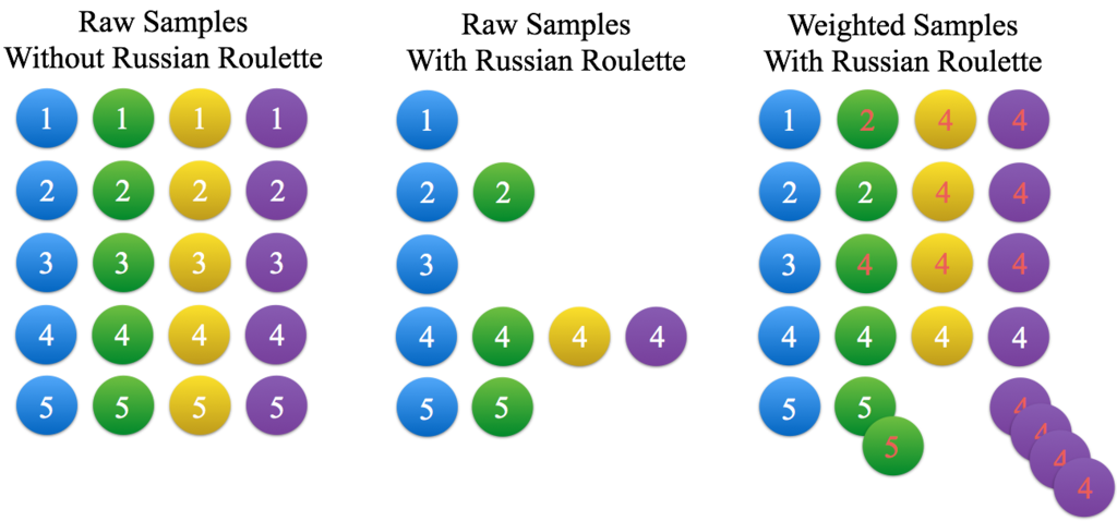
Shortly put, the Russian Roulette sampling technique can be interpreted as making "copies" of high-order terms, to use in place of the dropped off terms that were not evaluated in other samples. This can be described graphically using the following figure.

f:id:woodrush:20150725201736p:plain

Let us consider a problem where we want to evaluate 4 orders of some value, with 5 samples. In ray tracing, this could be evaluating the radiance using terms of up to 4 reflections with 5 samples, for instance. In the figure above, the colors correspond to the orders of the value, and the number n in the circle indicates that it is the n-th sample.

The leftmost figure shows a direct method of evaluating this value, that is to just simply evaluate all of the orders in all of the samples. However, in ray tracing it can be time-consuming to do such evaluations.

This is where the Russian Roulette sampling technique comes in. In the Russian Roulette technique, we aim to evaluate only a few high-order terms. Basically, before evaluating each order of terms, we roll some dice - and proceed to evaluate high order terms at only a given probability, or else halt the evaluation and move on to the next samples. Each higher order term must survive this judgement before it gets evaluated, or otherwise the "game" (higher-term evaluation) ends and moves on to the next round (sample) - therefore, the name "Russian Roulette." In this figure, we've assumed a 50% probability of proceeding to evaluate the next higher order. The figure on the center shows the actually calculated terms in each sample, for the Russian Roulette. In other words, the circles in the figure are the circles that "survived" the Roulette. Notice that the number of evaluations is reduced to around half of that in the left figure, and many high orders are dropped off.

Now, since we have excluded many orders, we don't have enough circles (terms) to add up to calculate the average. (i.e., simply taking the average of all of the terms (circles) provides an inaccurate estimate of the true value, compared to the estimator shown on the left figure.) Specifically, each n-th order term shows up at a ratio of (1/2)^(n-1) compared to the number of them in the left figure.

How do we calculate the average with such few circles (terms)? The answer, which is the Russian Roulette sampling technique, is to use copies of other circles (terms) as placeholders. Mathematically, the technique is to divide the value of each evaluated term by the probability of its appearance when taking the grand average. This obscure technique can be understood by observing the right side of the figure. Dividing the term by its survival probability p is equivalent to considering as if 1/p copies of that term has existed in the evaluation. This is the whole idea of the sampling technique, and is depicted in the figure above as copies of the circle. (Copies are indicated by red index numbers.) By making "copies" in such a way, the number of samples of each order approximately match that of the direct technique shown in the left side of the first figure. Although the number of circles differ from its true value (they are short in the 3rd order and excessive in the 2nd and 4th order), if we take a sufficient number of samples, the law of large numbers helps us to diminish those discrepancies to an ignorable level. Therefore, the "magic" of dividing higher order terms in the Russian Roulette technique, can be interpreted as making the "right number of copies" of that term, so that it properly compensates for the higher order terms that did not survive to be evaluated (i.e. dropped in the sampling process).

MATLABで、for文・parfor文中で関数内のパラメータを様々に変えて計算をする方法(クロージャの利用)

たとえば以下のような状況があると思います。

  • ある微分方程式の解軌道を、for文中で異なるパラメータごとに描きたい
  • ある方程式の解を、for文中で異なるパラメータごとに求めたい

このようなとき、ode45やfsolveを使いますが、for文中で関数の中身のパラメータの値を直接いじることはできません。

あまりよくない方法(parfor内では使えない方法)

そのため、たとえばglobalを使ってグローバル変数を定義し、関数内から変えたりする方法を取ったりします。例として、関数odefunc内のpという変数を様々に変えてode45をする場合、次のようになります:

% odefunc.m
function ret = odefunc(t,x)
    global p;
    ret = [-p*x(2); x(1)];
end
% main.m
global p;
for p = 1:10
    [t, y] = ode45(@odefunc, linspace(0,10,100),[1; 1]); 
    figure;
    plot(t,y);
end

この方法は比較的簡単ですが、parfor内では使えないという重大な欠点があります。parforはfor文と同じ文法で簡単に並列計算・高速化を行うための方法(MATLABのparforの使い方メモ(高速化のために) - woodrush’s diary 参照)なのですが、globalな変数を用いていると並列計算が行えないため、この方法が使えません。

良い方法 - 「関数を返す関数」を使う方法(parfor内で使える方法)

これは、「関数を返す関数」を使うとかなり綺麗に解決することができます。まずはソースを見てみましょう:

% odefuncFactory.m
function retfunc = odefuncFactory(p)
    function ret = odefunc(t,x)
        ret = [-p*x(2); x(1)];
    end
    retfunc = @odefunc;
end
% main.m
parfor p = 1:10
    odefunc = odefuncFactory(p);
    [t, y] = ode45(odefunc, linspace(0,10,100), [1; 1]); 
    figure;
    plot(t,y);
end

ここでodefuncFactoryという怪しい関数が出てきました。これはその名の通り、「パラメータpを与えると、そのpを使ったodefuncを返す関数」つまり「関数を返す関数」になっています。main.mの3行目にて、odefuncFactoryに所望のpを入れ、そのpを使ったodefuncを受け取っています。「odefunc = 」と書くことで、返ってきた関数をodefuncという変数に格納しています。(このように、MATLABでは関数も変数のように扱うことができるのです。)受け取ったodefuncをode45に渡し、シミュレーションを行っています。

この方法を使うと、異なるpごとに異なる関数を毎回作成することになるので、parfor内でも使えるようになるのです。このことを強調するために、2つ目のmain.mではfor文をparfor文にしました。

おまけ - 更に簡潔に

odefuncの程度のような短い関数ならば、無名関数を使うと更に短く書くことができます:

% main.m
odefuncFactory = (@ (p) (@ (t,x) [-p*x(2); x(1)]));
for p = 1:10
    odefunc = odefuncFactory(p);
    [t, y] = ode45(odefunc, linspace(0,10,100), [1; 1]); 
    figure;
    plot(t,y);
end

% 更に短く
parfor p = 1:10
    odefunc = (@ (t,x) [-p*x(2); x(1)]);
    [t, y] = ode45(odefunc, linspace(0,10,100), [1; 1]); 
    figure;
    plot(t,y);
end

main.mだけになってしまいました。一つ目の例のように、無名関数も「関数を返す関数」の作成に使えます。更に、odefuncくらいの関数なら、odefuncFactoryを作るまでもなく、二つ目の例のように直接odefuncを無名関数で構成することもできます。
ただし、最初の例では無名関数odefuncFactoryをparfor内で定義しているという違いに注意して下さい。無名関数を使うと何かとparforの制約に引っかかりやすくなるので、通常は個別のmファイルを作ることをおすすめします。

もう少し詳しく

この一連方法では「関数を返す関数」よりも、クロージャという概念が本質的に活用されています。2つ目のmain.mを見てみましょう。main.m中には「odefuncFactory関数の中にodefunc関数が包まれている」という階層構造があることに注目して下さい。次に、odefuncFactory.mのソースをよく見ると、「function ret = odefunc(t,x)」の中には変数pの定義が含まれていない(p= ... と書いていない)ことに気づきます。普通ならばどこにもpの定義が書いていなければエラーが起こります。それでも動くのは、odefuncの外のodefuncFactoryでpが定義されているからです。odefuncは、その外のodefuncFactoryに存在する変数pの値が「覗ける」ので、このプログラムは動くわけです。つまり、odefuncFactoryは、odefuncと共に、odefuncの外側の変数たちの知識、つまり外側の環境へのアクセスも与えています。このように、関数とその外側の環境のペアをクロージャと言います。odefuncFactoryは「関数を返す関数」と言いましたが、更に正確に言うと「クロージャを返す関数」だったわけです。

このようにMATLABの無名関数はクロージャを返してくれるという性質から、色々とマニアックなことができます。たとえば、条件分岐や複数行実行などが行えたりします。詳しくはMATLABの無名関数内で条件分岐・複数行実行を行う方法 - woodrush’s diaryを御覧ください。

MATLABのparforの使い方メモ(高速化のために)

MATLABのparfor構文を使うと、parfor内の処理を並列で行ってくれるため簡単に高速化ができます。たとえば多くのパラメータに対するシミュレーション結果を得たいとき、parforを使うと各パラメータに関する計算を簡単に並列化することができます。

しかし、parfor内の処理には、並列化のためのやっかいな制限があります。中でも「結果を配列に書き込むときは、異なる並列計算の書き込み先インデックスが競合しないことが保証されなければいけない」という制限がくせもので、これ自体は当たり前な事なのですが、これをMATLABに納得させるようにプログラムを書くのが少し面倒だったりします。
以下に、parforがちゃんと動くコードを示します。内容は、ある2パラメータtheta1とtheta2の直積の範囲で計算を走査するプログラムとなっています。

% 走査したいパラメータ
theta1 = 1:100;
theta2 = 1:100;

% parfor内から書き込みたい配列のサイズを、parforのインデックスの最大値として明示する
resultMatrix = zeros(length(theta1),length(theta2));
theta1indmax = size(resultMatrix,1);
theta2indmax = size(resultMatrix,2);
% theta1ind, theta2indを陽にインデックスに指定する・その1
parfor theta1ind = 1:theta1indmax
    for theta2ind = 1:theta2indmax
        % theta1ind, theta2indを陽にインデックスに指定する・その2
        resultMatrix(theta1ind,theta2ind) = theta1(theta1ind)^2 + theta2(theta2ind)^2;
    end
end

contourf(resultMatrix);

% parfor中で配列に書き出さない時は、上記の制限を気にせず書くことができる
parfor theta1ind = 1:length(theta1)
    for theta2ind = 1:length(theta2)
        [theta1(theta1ind) theta2(theta2ind)]
    end
end